Home | About | Apps | Github | Rss
Introduction to R language
Inspired by a friend’s prolific use of R for doing data analysis, over past few days I have been trying to get the hang of the language. Here are some notes and thoughts
First impressions
Thinking of R as a programming language may sub-consciously invite a notion of procedural logic. That was a path not worth going down. Its easier to assimilate the syntax, if one were to consider it an expression evaluation system.
Not having worked with any kind functional languages (unless you consider javascript), I had to find analogies to the procedural world, to help grasp the fundamentals.
Here are my notes starting from the very basics to the point of being able to make a basic plot.
Docs
Am following documentation here - https://cran.r-project.org/doc/manuals/R-intro.html. For the most part, it is great, although some parts may seem tediously verbose, fretting on about smallest details.
Getting Started - IDE
R Studio is a pretty good place to start learning and using R. It features.
- REPL (interactive prompt)
- Notebook from which you can execute one or many statements into your REPL.
- package manager
- Graphics/output viewer
- Variable viewer
REPL
Python’s REPL allowed me to learn the language without leaving the convenience of the terminal and in the absence of internet a decade ago in India.
R’s REPL in R-Studio takes it a notch further.
Getting help is quite easy. Simple executing ?func will open docs for that function.
> ?plot
Types
The language is loosely typed. Variables can be assigned to one type and re-assigned to another later.
> a = "foo"
> class(a)
[1] "character"
> a = 23
> class(a)
[1] "numeric"
R being primarily a statistical analysis language, the primitive data types are quite diverse. A non-exhaustive list for an idea:
- numeric
- complex
- character (strings)
- vectors (think arrays)
- matrices
- factors
- data frames (think tables)
- etc
Assignment
Variables are assigned from right to left with either = or <-. You can also perform left to right assignments by the use of -> operator.
> a <- 23**2
> 23**2 -> a # assign expression into a
> print(a)
[1] 529
Vectors
Closest (and insufficient) analogy is to think of them as arrays, but richer.
create vectors
A vector can be initialised using c()
> c(1,123,33,223,2) -> a
> print(a)
[1]   1 123  33 223   2
> sum(a)
[1] 382
All elements of the vector must be of the same type. If elements all but one are numeric and last is string, all are coerced to become a string
> c(1,2,3,"f")      # all but one are numeric
[1] "1" "2" "3" "f" # all coerced to strings
> c(1,2,3,"f") -> a
> class(a)
[1] "character"
c() function flattens nested vectors
> c(a, c(1,2,3))
[1] "1" "2" "3" "f" "1" "2" "3"
length and indexing
Length can be computed using length() function.
Items can be accessed using a one-index notation.
> a
[1] "1" "2" "3" "f"
> a[1]
"1"
range of elements
Range of items can be expressed as variable[from: length]
> a
[1] "1" "2" "3" "f"
> a[0:2]
[1] "1" "2"
Numeric vectors can also be created using the range syntax
> 1:10
 [1]  1  2  3  4  5  6  7  8  9 10
out of bounds
Index can go out of bounds. Out of bounds elements will be marked with a typedNA value.
> a
[1] "1" "2" "3" "f"
> a[0:10]
[1] "1" "2" "3" "f" NA  NA  NA  NA  NA  NA
expression selection
a[<expression>] can contain any valid expression and is not limited to range representation
> b = c(1,2,3,NA,NA) # consider
> b[b>2]             # elements of b > 2
[1]  3 NA NA

> b[ !is.na(b) ]     # elements of b that is not `NA`
[1] 1 2 3

> b[ b > 2 & !is.na(b) ] # b > 2 and that is not `NA`
[1] 3
using operators
Any basic math operation performed, is applied to whole vector and result is represented as an equivalent vector.
> b = c(1,2,3)   # assign
> b
[1] 1 2 3
> b + 1          # +1 all elements
[1] 2 3 4
> b*b            # square all elements
[1] 1 4 9
Addition of multiple vectors will result in one-to-one addition.
> c <- 1:5                  # c = c(1,2,3,4,5)
> d <- 6:10                 # d = c(6,7,8,9,10)
> c + d
[1]  7  9 11 13 15          # 1+5, 2+6
vectors of in-equal can participate in binary operations - the catch being the shortest vector will be repeated
> 1:6 -> p        # 1 2 3 4 5 6
> 1:3 -> q        # 1 2 3
> p + q
[1] 2 4 6 5 7 9   # 1+1, 2+2, 3+3, 4+1, 5+2, 6+3
labels
Elements of a vector can be named
> x = c(foo=1,2,3,4,5)  # named vector element
> x
foo                     # column name
  1   2   3   4   5
It can be accessed both by an index as well as by its name.
> x[1]
foo
  1
> x["foo"]
foo
  1
The names can be obtained by names function.
> names(x)
[1] "foo" ""    ""    ""    ""
Plotting a simple vector
Consider vectors
> x = 1:5
> x
[1] 1 2 3 4 5
> x^3
[1]   1   8  27  64 125
Plotting x vs x^3 is as simple as running the function plot()
> plot(x = x, y = x**3, type='b')
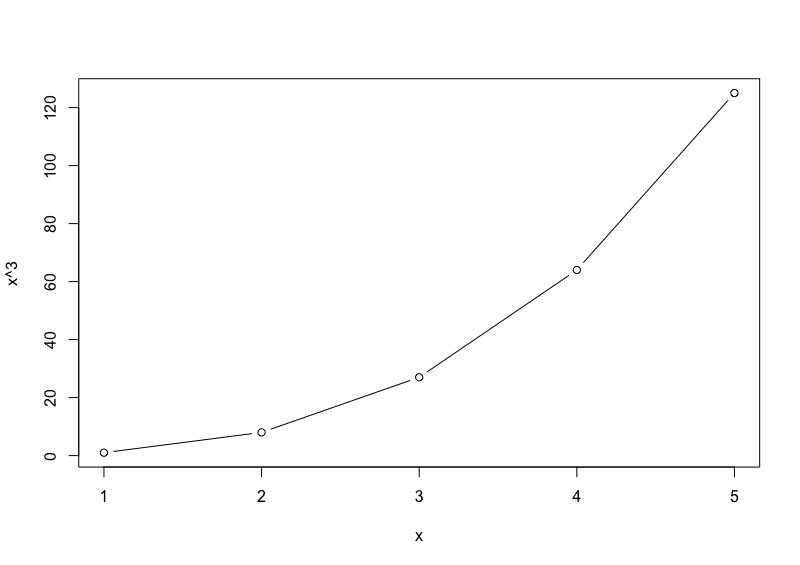
Note on the parameter type:
- ‘b’ - indicates “both” points and lines
- ‘p’ - will plot only points
- ’l’ - will plot only lines
More posts
- Next: Books in 2017
- Previous: Getting started with a blank iOS Project